Automating Digital Twins Implementation In Downstream Bioprocessing

By Daniel Espinoza, Ph.D., Lund University

Developing a downstream process for a new drug candidate is a costly task precisely because of the high value of the potential drug. While, traditionally, this development is performed by selecting and executing experiments in a laboratory at small scales, the advent of digital tools, particularly mechanistic models, enables the process developer to forego the laboratory and perform a multitude of experiments in silico, i.e., in a digital environment, saving time and resources.

A mechanistic model, that is, a mathematical set of equations that aim to accurately predict the physical and chemical interactions in a process system, can be used in conjunction with other advanced computational and mathematical tools to provide rapid development of novel, optimized downstream processes.

However, a mechanistic model does not eliminate the need for laboratory experiments. In particular, having real-world data to compare the model with is crucial: a model is only useful if it is able to predict something about reality. Selecting a set of experiments to generate such data, while keeping the number of experiments as low as possible, is in itself a difficult task, not to mention selecting mathematical equations that accurately represent the system of interest. This creates a dilemma where the work required to generate a mechanistic model, or digital twin, of a downstream process system can be seen as excessive in an environment where many drug candidates need to be screened in a short amount of time.

Thus, the question: can we somehow automate the work in generating a digital twin? To address this, my colleague Simon Tallvod and I set up a small case study on an ÄKTA Pure chromatography system (Cytiva, Uppsala, Sweden). Building on his previous work (Tallvod et al., 2022), we set out to create a workflow that would take the user from a fresh chromatographic setup to a complete digital model of the system and a suggested operating point for performing the chromatographic separation. To this end, we identified the following necessary steps:

1. Create a mathematical system of equations to represent the entire chromatography system.
2. Perform a set of experiments to generate necessary data for model calibration.
3. Import the data into a computer program.
4. Perform model calibration using the generated data.
5. Use the model to suggest an optimal operating point.
6. Validate the model and optimal point to ensure that it works.

Using Python To Link Workflows And Modeling

The key to being able to achieve automation of this workflow was a piece of software called Orbit, built at the Division of Chemical Engineering at Lund University in the Python programming language. Orbit is an automation tool that can be used to manipulate laboratory equipment via Python scripts, which it achieves by accessing the equipment’s communications interface.

For instance, in the context of ÄKTA chromatography systems, it can be used to switch valves to different positions, set pump flow rates, and obtain measurements from the in-line UV absorbance and conductivity sensors. In Python code, the user defines the components of the instrument, such as valves, tubing, pumps, columns, and sensors present by pulling them from a Python object library built into Orbit. These Python objects contain small functions that correspond to different control actions in the system, such as setting the flow rate of a pump.

The user can then write sequential instructions in a Python script and, by running that script, the instructions will be executed in order. The main benefit of Orbit is that it allows the user to perform tasks that may not be enabled by the proprietary control software that comes with the equipment, as well as the ability to automate said tasks.

For the task of automating the modeling workflow, we extended Orbit’s functionality to include mathematical equations corresponding to the mass transport in each type of equipment. These equations were then added to a system of equations automatically as Orbit reads through the system configuration defined by the user. This means that by simply using Orbit in the standard way, a digital system of equations has already been created, and we have achieved step 1 of the modeling workflow.

For an illustration of the system configuration used in our case study, see Figure 1.

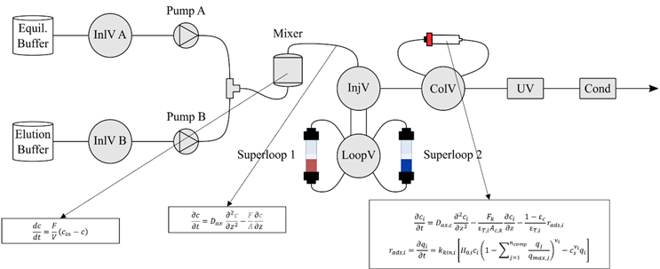
Figure 1: The system configuration used in the automatic modeling case study. Orbit was used to automatically build a system of equations based on the user-defined components. Example equations are shown for a mixer, a piece of tubing, and the chromatography column. The column was placed on the column valve, and two superloops were placed on the loop valve, each containing a sample mixture used in the experiments performed to generate data for model calibration. Adapted with permission from (Espinoza et al., 2024).

Push-Button Modeling For A Completed Data Set

Step 2 was automated using the standard Orbit functionality of automatically performing experiments based on predefined scripts. Using existing knowledge about data generation for chromatography systems, in particular, for ion-exchange chromatography, a set of six experiments was preprogrammed in Python. Each experiment was then executed in sequence, meaning that once the scripts were predefined, the user merely pressed “play,” left the lab, and returned a few hours later to a completed data set.

In order to automate the experiments, the two superloops shown in Figure 1 were essential. Superloop 1 contained a protein sample representing a biopharmaceutical to be purified. In our case, this was a cytochrome C solution containing multiple size and charge variants of the protein, where one was the intended target for purification. This sample was used to perform bind-and-elute experiments on the chromatography column, which yielded information about the binding properties of the protein and the impurities.

Superloop 2 contained a mixture of acetone and blue dextran, which was used to estimate the dead volumes of the column. By placing the samples in superloops, we were able to circumvent the issue of having to manually prepare the samples in the system prior to each experiment.

The automation of step 3 was implicitly solved by using Orbit: thanks to the direct communication between Orbit and the sensors of the ÄKTA system, we obtained data from the sensors directly into Python, which made it available for step 4, model calibration.

Multiple Experiments Lead To Optimal Process Design

In chromatography, model calibration, i.e., the fitting of model parameter values to experimental data, is commonly done using nonlinear curve fitting techniques. To fully describe the chromatography system, we divided the model calibration into several segments, six in total, each using different parts of the data generated in step 2 to fit simulated chromatograms.

A summary of the calibration steps, the parameters they estimated, and the experiments from which they used data is shown in Table 1.

Table 1: Summary of calibration steps, samples used in each step, experiments required, parameters estimated, and number of parameters estimated per step.

Step	Sample	Experiment	Purpose	Number of parameters
1	Protein mixture	System pulse experiment	System dead volume	1
2	Acetone + blue dextran	Column pulse experiment	Column void	1
3	Acetone + blue dextran	Column pulse experiment	Column porosity	1
4	Protein mixture	Linear gradient experiment x 3	Initial estimation of adsorption kinetics	3 x m, where m is the number of components
5	Protein mixture	Linear gradient experiment x 3	Adsorption kinetics + component concentrations	4 x m, where m is the number of components
6	Protein mixture	Overload experiment	Adsorption capacity	m, where m is the number of components

 

By estimating a dead volume excluding the column, any extra residence time effects introduced by tubing and other components of the system could be separated from the actual column dynamics, meaning that less error was introduced into the adsorption parameters.

One of the main benefits of a mechanistic digital model of a process like this is the ability to perform a large number of experiments for design of an optimal process. By using nonlinear programming techniques, we used the calibrated model for step 5, with the design being a linear gradient elution process that would maximize process yield and productivity while respecting a minimum purity requirement. The design variables were the initial mobile phase concentration during elution, the slope of the linear gradient, and the volume of the protein sample loaded on the column. The resulting process parameters that resulted in optimal performance were then made accessible to the user.

However, there is no guarantee that a suggested optimal operating point obtained from in silico studies will result in a feasible separation. The purpose of step 6 was to validate both the model and the suggested operating point by repeating the separation in the physical system. Even this can be performed as part of the automated workflow, since Orbit has access to both the optimization results and the physical laboratory setup. Based on the results from this validation experiment, the user can then decide whether to proceed with the obtained model or to take a step back and refine it.

Conclusion

For our small case study, this procedure worked quite well. The optimum that was suggested by the framework resulted in a good enough model fit for additional process development. However, this was a study on a single chromatography purification step. In a real-world scenario, multiple process steps could benefit from modeling and optimization using this framework. At the moment of writing, work is underway at the Division of Chemical Engineering at Lund University to apply this same modeling framework on multicolumn chromatography purification of a monoclonal antibody. One could also easily imagine it being applied to other important process unit operations, such as membrane filtration. Thanks to the flexibility of Orbit, expansion to include these additional unit operations is a relatively simple matter.

It might be easy to perceive this case study as an endorsement of Orbit. While very flexible and extremely useful, I would like the reader to take the following message to heart instead: the only reason that Orbit is as powerful as it is, is that the hardware developers with whom we have worked have had open communication protocols that we could access with Python.

Many hardware suppliers choose to have closed communications interfaces, and I can definitely understand the reasons for that. However, I would like to deliver the, admittedly naïve, message that for innovation in modeling and automation to take place, these open protocols are a must. They allow for incredibly novel approaches to process development.

About The Author:

Daniel Espinoza, Ph.D., is a chemical engineer and researcher at Lund University focusing on the automation and digitalization of biopharmaceutical production processes through modeling, simulation, and process control.