Cleaning Process Capability: Understanding Populations, Samples, And Sample Size Requirements

By Andrew Walsh; Thomas Altmann; Joshua Anthes; Ralph Basile; James Bergum, Ph.D.; Alfredo Canhoto, Ph.D.; Stéphane Cousin; Hyrum Davis; Parth Desai; Boopathy Dhanapal, Ph.D.; Jayen Diyora; Igor Gorsky; Benjamin Grosjean; Richard Hall Hall; Ovais Mohammad; Mariann Neverovitch; Miquel Romero-Obon; Jeffrey Rufner; Siegfried Schmitt, Ph.D.; Osamu Shirokizawa; Steven Shull; Stephen Spiegelberg, Ph.D.; and John VanBershot

Part of the Cleaning Validation For The 21st Century series

This article is the fifth in a series on process capability that started with a primer,¹ then a statistical examination of cleaning data collected using total organic carbon analysis,² followed by an examination of how to evaluate cleaning data that is partially below the detection limits³ or completely below the detection limits.⁴ This article will examine the role of sample sizes in the determination of process capability or process performance.

What Is A Population?

In statistics, a population includes all individuals that share a specific characteristic that you are interested in studying. This information can be achieved by measuring every member of the population, which is called a census. In many cases the population may be so large that we cannot measure every member of the group in an economic or efficient manner. In these cases, we can take a sample, which is a portion or a fraction or a percentage of the population. From such a sample, well established statistical techniques can provide us with important information about the population sampled.

For example, the population of interest might be the entire surface of a piece of equipment that was cleaned according to a specific cleaning procedure (i.e., a cleaning SOP). Figure 1 shows a graphic illustrating this concept. In this example, the entire surface area of a V-blender with an area of 250,000 cm² can be represented as a population of 10,000 smaller areas of 25 cm² size (Figure 2), which is the total area of a 5-cm x 5-cm swab area.

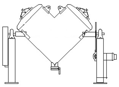
Figure 1: Hypothetical pharmaceutical blender with a total surface area of 250,000 cm²

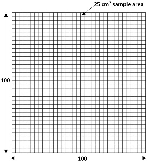
Figure 2: Map of the hypothetical pharmaceutical blender with a population of 10,000 25 cm² sample areas

In cleaning validation, we typically want to know the cleanliness of the entire surface of a piece of equipment. Ideally, we would like to know that every area of the entire surface is as clean as any other area. We can determine this by testing the entire surface area of the equipment. We could test, for example, all 10,000 of these smaller areas for total organic carbon. However, it is generally considered impractical, if not impossible, to test the entire surface area of the equipment. Rather than test each area, we can take samples of this population and, using well recognized statistics, we can draw conclusions about the entire population from these samples. A statistical sampling plan can be used to assure the cleanliness of the blender across the entire surface by sampling a subset of the 250,000 cm²s. Such a sampling plan requires knowledge of two important concepts: sampling distributions and the central limit theorem, which are discussed in the following subsections.

Sampling Distributions

A sampling distribution is the distribution of a statistic (e.g., the mean) that is found from repeated samplings of n members of the population following a sampling plan. Each member sampled (i.e., the individual 5-cm x 5-cm or 25 cm² swabs) is tested to obtain a numerical result (e.g., total organic carbon as a measure of cleanliness). The results are assumed to follow a distribution. The most common distribution is the normal distribution. The results are used to estimate the parameters of the normal distribution, which are the mean (μ) and the standard deviation (σ). The mean and standard deviation define the normal distribution that can be used to tell us important and useful information about the other members of the population that we have not sampled or measured. This information allows the user to draw valid conclusions about the population. As an example, suppose the “true” mean (μ) and standard deviation (σ) of TOC are 150 ppb and 25 ppb, respectively. The blue curve in Figure 3 shows the distribution of single results (i.e., means of n=1).

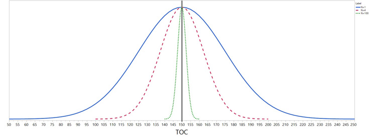
Figure 3: Normal distributions of means based on sample sizes of one, four, and 100

Note that the distribution is centered at μ=150 ppb. Sixty-eight percent of distribution means will always be within one standard deviation of the mean and 95% will fall within 1.96 standard deviation of the mean. So, on the blue curve based on a sample mean based on one result, about 68% will fall between 125 ppb and 175 ppb and 95% will fall between 101 ppb and 199 ppb). In this example, the standard deviation of individual results is 25 ppb, but if the standard deviation of the individuals was smaller, all of the curves would be tighter.

The sample mean is the average of n individual results. Figure 3 also shows the distributions of means based on sample sizes of n = 1, 4, and 100. The distribution of means based on four results is shown by the red curve and the distribution of means based on 100 results is the green curve. As can be seen from these curves, the distribution of the mean depends on the sample size. The curves for any sample size will always be centered at μ=150 ppb but the standard deviation of the mean becomes smaller as the sample size increases. It makes intuitive sense that this will happen since the mean of four randomly single results from the blue curve (n=1) would tend to have results scattered about the population mean so that the mean of the four results would tend to be closer to the population mean, resulting in a tighter distribution (i.e., smaller standard deviation), as shown in the red curve. The relationship between the standard deviation of the individual data (n=1) and that of a mean based on a sample size of n is always σ/√n (e.g., for n=4, 25/√4 = 12.5 ppb). As stated above, 68% of means will be within one standard deviation of the mean. In the example, this is ± 25 ppb for the individuals, or 12.5 ppb for n= 4 and 2.5 ppb for n =100. About 95% will fall within 1.96 standard deviations. So, for example, with a sample size of four, about 68% of the means will fall between 137.5 ppb and 162.5 ppb (i.e., 150 +/- 12.5).

Central Limit Theorem

In the previous section, we assumed that the data was normally distributed. What if the distribution is not normal? A very important characteristic of the mean sampling distributions is that the means of samples will follow a normal distribution — no matter what type of distribution the samples are taken from as long as the sample size is large enough. This characteristic is described in the central limit theorem.

The central limit theorem is an important and fundamental principle that underlies many of the statistical analyses that are performed on a daily basis, including confidence intervals and control charting, and it has applicability to cleaning data.

In simple language, what the central limit theorem tells us is that: The means of samples ( ) will tend to follow a normal distribution regardless of what type of distribution the samples are taken from (if the sample size is large enough). See Figure 4.

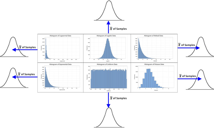
Figure 4: Graphic showing the sampling distribution of the means of samples from several distributions. The graphs above show the histograms of 100,000 individual data points to show the shapes of their distributions. If samples and the sample mean (based on a large enough sample size) are calculated for each sample, the means from any of these distributions (blue arrows) will be normally distributed. This will be true even for the extremely non-normal distributions (like the exponential or the uniform) if the sample size is large enough. Figure modified from Walsh, Andrew: Cleaning Validation - Science, Risk and Statistics-based Approaches, 1st Edition (2021), used with permission.

There are three important points to realize from the central limit theorem:

1. The mean of the sampling distribution of means is equal to the mean of the population the samples are from.
2. The standard deviation of the sampling distribution of means (the standard deviation is the standard error of the mean or ) is equal to the standard deviation of the population the samples are from divided by the square root of the sample size (n).
3. For normal populations the sampling distribution of means will be normal AND for non-normally distributed populations the sampling distribution of means will become increasingly normal as the sample size increases. This is particularly true for distributions like the uniform and exponential, where larger sample sizes (e.g., >30) are needed (another origin for the n=30 requirement myth). Therefore, you can confidently sample from any kind of distribution shape and be assured that the sampling distribution for the mean will follow a normal distribution if the sample size is large enough. This allows us to use statistical processes and functions for normal distributions. In addition to this, cleaning validation samples generally should be normally distributed.²

This understanding can allow scientifically justifiable conclusions to be made about the cleanliness of the entire equipment, and of the performance of the cleaning process, based on our sample data. So, if we know the mean and standard deviation of our samples we can calculate how many members of the population are above or below a certain value (such as an acceptance limit). Knowing this fact allows us to calculate the process capability, or the process performance, of a cleaning process from a sample (Figure 2).

Sample Size

There has been much written about the importance of sample size in statistics. Many pharmaceutical workers (validation, QA, regulatory affairs, operations, etc.) have been challenged to make even a simple decision for fear of not having enough data. While it is commonly understood that larger sample sizes lead to increased accuracy when estimating unknown parameters, a minimum sample size of say, 30, is not a requirement for meaningful statistical analysis. However, less than four can make confidence intervals wider than desired. While more sample data is always better, there are many circumstances (such as can be found in cleaning validation) where even a small number of samples can provide more than satisfactory information. The following examples will show how this is normally the case for cleaning validation samples.

In the blender example above, how many samples do we need to take to achieve an acceptable level of confidence that these samples represent all the other sample areas of the equipment? As we will see, that depends on how confident we want to be that the samples are less than the acceptance limit and this is also directly dependent on the level of the acceptance limit.

Our ability to rely on the value we get from the process capability or process performance calculation (confidence intervals) depends on the number of samples we have taken (n). Conversely, we need to know the number of samples required (sample power) to achieve an acceptable confidence interval.

Confidence Intervals

The actual value of a statistical parameter (e.g., mean) of any population is never truly known and is only estimated from the sample data collected. More often than not, testing an entire population is not economical, reasonable, or possible, so sampling is necessary. For example, in cleaning validation, swab samples are not taken from every cm² of an equipment surface and the mean of several swab samples is accepted as representative of the entire equipment surface. But this mean is only an estimate of the true value and it would be helpful to know how much confidence we can have in that mean.

A range of possible values for the statistical parameter can be calculated from the sample data, and this is called a "confidence interval." A confidence interval refers to the probability that the confidence interval will capture the statistical parameter for a population. Analysts often use confidence intervals that contain the parameter of either 95% or 99% probability. What this means for cleaning validation samples is that you can be 95% or 99% confident that the confidence interval will contain the population parameter. Figure 5 below shows the equation for calculating confidence intervals.

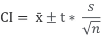
 = Sample Mean
t  = t-score (e.g., for 95%, 99% confidence interval)
s = Standard Deviation
n = Number of Samples

Figure 5: Calculation of Confidence Interval (CI): The CI is calculated using values that we know from our sample data: the sample mean (), the standard deviation (s), and the sample size (n). The confidence level we want (e.g., 90%, 95%, 99%) is obtained from a table of t-scores. The t-score is simply the number of standard deviations a data point is away from the mean. It is based on the sample size n. As the sample size increases, the t-value gets closer to a z-score. The most common z-scores are well known to people familiar with statistics. For example, the z value for 95% = 1.96 and for 99% = 2.576 (these scores are simply used for convenience as two standard deviations would be 95.45% and three standard deviations would be 99.73%). The CI is calculated from the t-score, s, and n and added and subtracted from the to obtain the possible range for the population mean difference. It should be understood that the larger the sample size (n), the smaller this range will be (also t).

Using the TOC example, Table 1 shows the 95% confidence intervals based on sampling three, five, 10, and 30 samples generated from a normal distribution with a population mean of 150 and a standard deviation of 25. Note that the sample means and standard deviations are "point estimates” of the population mean and standard deviation. All of the 95% two-sided confidence intervals captured the population mean of 150.0 ppb. We would expect that if a large number of samples were drawn and 95% confidence intervals were generated, 95% of them would capture 150.0 ppb. Note that although there is only one sample for each sample size, as expected, the range of values becomes smaller and smaller as the sample size increases. On average, increasing the sample size from three to 30 will reduce the width by over 70% using the formula above, due to dividing by √30 instead of √3 and using a smaller t value.

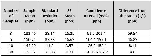
Table 1: Confidence intervals for samples from a population with a mean = 150 ppb and standard deviation = 25 ppb.

Figure 6 provides a graphical plot of the data in Table 1.

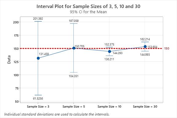
Figure 6: Confidence Interval Plot for Sample Sizes of three, five, 10, and 30: Note that the true mean for the population (150.0 ppb) is contained within each confidence interval.

The 95% confidence interval for the underlying mean with a sample size of three is 61.5 ppb to 201.4 ppb. This means the underlying population mean could be anywhere between 61.5 ppb and 201.4 ppb. If the goal was to show that the population mean of the batch is less than 300 ppb, then the confidence interval supports this goal. But the interval would not support that the population mean is less than 180 ppb, since 180 ppb is within the confidence interval, even though the sample mean was only 131.46 ppb. The confidence interval based on a sample size of 10 would support that the population mean is less than 180 ppb. The sample size of three resulted in too wide a confidence interval to accurately estimate the population mean due to sample size and the high standard deviation. If a tighter confidence interval is desired, then the sample size needs to me increased. Deciding on a sample size requires performing a power analysis, which is discussed in the next section.

Confidence intervals⁶ are important in evaluating cleaning processes as the largest interval value (upper bound) is used as the worst case for determining the process capability score, as it will provide the lowest process capability score for that sample size. As discussed in the first article¹ the calculation of process capability for the upper limit (Cpu) is:

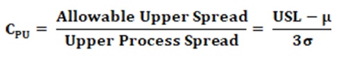
Figure 7: Calculation of Process Capability Index (Upper): Using the upper bound of the confidence interval in this calculation will decrease the value of the allowable upper spread, resulting in a lower C_pu result. Also, since C_pu is based on sample estimates μ and σ (i.e., sample mean and standard deviation), the larger the sample size, the closer the sample C_pu it is to the population C_pu. (A confidence interval for C_pu can be constructed but is not addressed in the document.)

While using the upper bound of the confidence interval to calculate the process capability provides a worst-case evaluation of the process capability result, it is important to confirm how reliable the sample size is in demonstrating that the sample mean is lower than the acceptance limit. This can be determined by calculating the power for a specific sample size.

Sample Power

In the previous confidence interval section, we were able to provide with 95% confidence a range for possible population means. For n = 3, the range was 61.5 ppb to 201.4 ppb. This indicates that any value for the population mean within that interval is possible. A statistical test that the population mean is = 200 ppb would be possible since it is contained in the interval or a test that the population mean is 65 ppb would also be possible. But a population mean of 200 ppb may be unacceptable. The wide interval is due to a large standard deviation and a small sample size. As seen in Table 1, all of the confidence intervals with a sample size greater than three do not contain 200, so we would conclude that if we wanted to test that the population mean was 200 ppb, we would reject it since 200 ppb is not within the confidence interval. We want a sample size that would accept an acceptable population mean but reject an unacceptable population mean. Power is performed prior to collecting data and performing the test. An estimate of the population standard deviation is needed, which may be determined from previous data. Power is the probability of rejecting a specific population mean. Suppose we want to statistically test that the population mean is 200 ppb (called the null hypothesis), but the population mean is really only 175 ppb, which is considered unacceptable (called the alternative hypothesis). We would want a high probability to reject that the population mean is 200 ppb. This requires determining a sample size that will accept the null hypothesis and reject the alternative hypothesis.

Example 1

A cleaning validation subject matter expert (SME) has an HBEL limit calculated for a new product being introduced to their facility at 525 ppb. The mean of the current cleaning data is 150 ppb (with a standard deviation of 25 ppb), so the difference between the new limit and the data mean is 375 ppb. The cleaning validation specialist wants to know if three swab samples would be enough to demonstrate that the cleaning process supports the new HBEL-based limit for this new product. The cleaning validation specialist runs a power curve using these parameters (Figure 8).

Based on the current cleaning data, the expected difference from the limit for the new product is 375 ppb. We want to test that the new process has the same difference. Therefore, the hypothesized difference is zero. But if the population difference is 375 ppb, we want to reject this hypothesis. We want a sample size that has a high probability of rejecting 375 ppb. This can be done by generating a power curve as shown in Figure 8 with a sample size of three. This power curve is based on a one-sided test (i.e., only interested in the upper value), an estimated standard deviation, and a null hypothesis α testing value of 0.01. The power is the probability of rejecting the null hypothesis for a specified difference. A commonly used probability for power is 80%, which would occur around 120 ppb and 140 ppb.

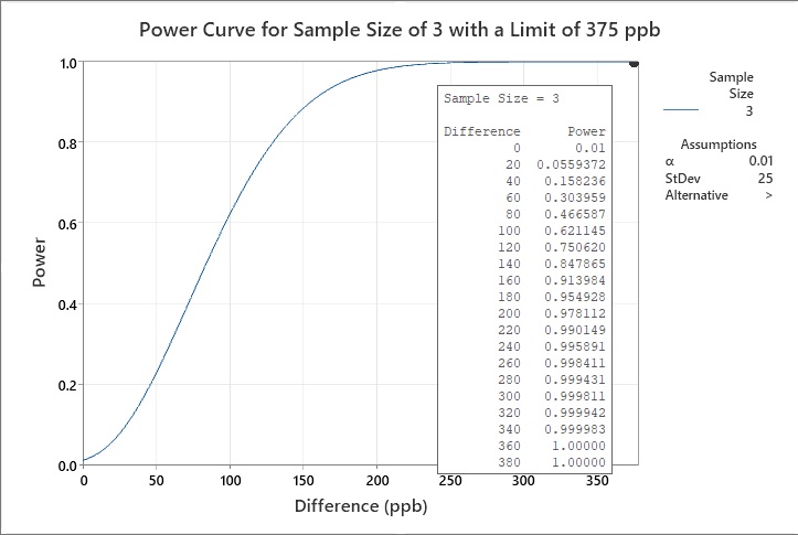
Figure 8: Example 1 of statistical power of a sample size of three with a limit of 375 ppb

The power curve in Figure 8 shows that the power at the 99% confidence level (α = 0.01) is 0.990149 for a difference of 220 ppb and jumps to 1 (100%) at 360 ppb. This indicates that a sample size of three is more than adequate for a difference of 375.

Example 2

Another cleaning validation SME has an HBEL limit calculated for a new product being introduced to their facility (250 ppb). The mean of the current data is 150 ppb (with a standard deviation of 25 ppb), so the difference is now only 100. The cleaning validation specialist wants to know if three swab samples would be enough to demonstrate that the cleaning process supports the new HBEL-based limit for this new product. This power curve (Figure 9) shows that the power (at a 99% confidence level) is 0.621145, a difference of 100, indicating that a sample size of three is poor.

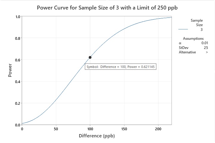
Figure 9: Example 2 statistical power of a sample size of three with a limit of 250 ppb

The cleaning validation SME then examines the power if six samples were taken. The new power curve (Figure 10) shows that the power (at a 99% confidence level) is 0.999971, a difference of 96, indicating that a sample size of six is sufficient.

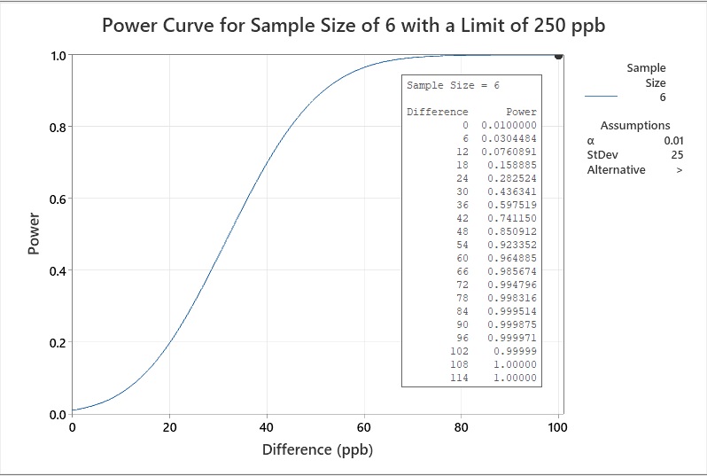
Figure 10: Example 2 Statistical Power of a Sample Size of six with a Limit of 250 ppb

Increasing the sample size will increase the power, but only to a certain extent. Once you have enough samples, every additional sample that is taken only slightly increases the power. Consequently, collecting more samples (e.g., 30) only increases the time, resources, and costs spent, without any additional benefit.⁷

So, rather than guessing, we can easily calculate the sample size if we know the mean and standard deviation of our cleaning data, have an acceptance limit to compare it to, and know what power we want or need.

Example 3

Another cleaning validation SME has an HBEL limit calculated for a new product being introduced to their facility (180 ppb). The mean of the current data is 150 ppb (with a standard deviation of 25 ppb), so the difference is only 30 ppb. The cleaning validation SME wants to know what swab sample size will be enough to demonstrate that the cleaning process supports the new HBEL-based limit for this new product with a power (at a 99% confidence level) of 0.99, for a difference of 30. Since the limit is very low, the SME wants to be very sure the data indicates appropriate cleaning. In this example the power curve indicates a minimum sample size of 18 (Figure 11).

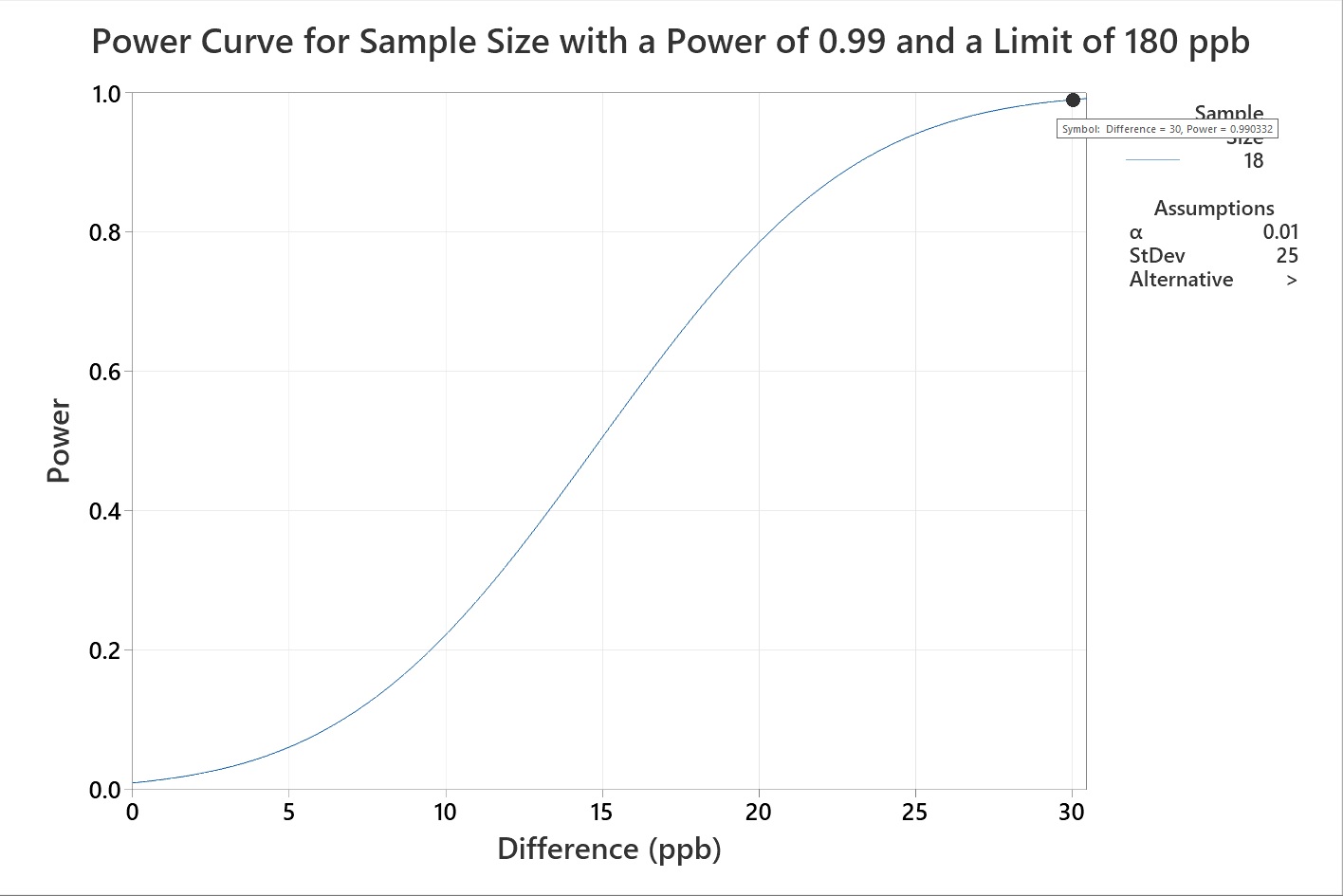
Figure 11: Example 3 of sample size to statistical power

It has been a common practice in the industry to only sample areas that are considered hard to clean or worst cases, but this practice may be arbitrary and not scientifically justified. For a science- and risk-based approach, a statistically appropriate number of samples should be taken. It is also recommended to “fingerprint” the equipment or medical device surface to establish a baseline of residue levels across all surfaces and not just those considered hard to clean or worst cases.

Summary

From this discussion we believe the reader should now be convinced that, based on the central limit theorem:

• The mean of the sampling distribution of means is equal to the mean of the population, and the standard deviation of the sampling distribution of means is equal to the standard deviation of the population the samples are taken from (divided by the square root of the number of samples).
• The means and standard deviations of cleaning samples can provide reliable information about the residue levels of entire equipment surfaces.
• Relatively small samples can provide a high degree of assurance that residues after cleaning processes are below acceptance limits.
• The number of samples necessary is dependent on how low the acceptance limit is and the statistical power desired.
• The number of samples taken should be statistically justified and not just for those considered hard to clean or worst cases (it should be noted at the same time that small sample sizes may be biased by one or two high results).

The understanding that cleaning process capability can provide a measure of the level of risk also can facilitate the implementation of the second principle of ICH Q9 and justify a "level of effort, formality and documentation commensurate with the level of risk" for the cleaning validation process.^9,10 The knowledge and understanding gained from such cleaning process capability estimates can even be used for justifying simpler analytical methods such as visual inspection.^11,12

In the next article in this series we will look at applying this understanding to selecting the number of cleaning process performance qualification runs and the optimal number of samples to take to minimize these runs.

Peer Review

The authors wish to thank Sarra Boujelben, Gabriela Cruz, Ph.D., Andreas Flueckiger, MD, Christophe Gamblin, Ioanna-Maria Gerostathes, Ioana Gheorghiev, MD, Cubie Lamb, Tri Chanh Nguyen, Ajay Kumar Raghuwanshi, and Basundhara Sthapit, Ph.D., reviewing this article and for providing insightful comments and helpful suggestions.

References

1. Walsh, Andrew, Miquel Romero Obon and Ovais Mohammad Calculating The Process Capabilities Of Cleaning Processes: A Primer, Pharmaceutical Online, November 2021
2. Walsh, Andrew, Miquel Romero Obon and Ovais Mohammad Calculating Process Capability Of Cleaning Processes: Analysis Of Total Organic Carbon (TOC) Data, Pharmaceutical Online, January 2022
3. Walsh, Andrew, Miquel Romero-Obon and Ovais Mohammad. Calculating Process Capability of Cleaning Processes with Partially Censored Data, Pharmaceutical Online, May 2022
4. Walsh, Andrew, Miquel Romero-Obon and Ovais Mohammad. Calculating Process Capability of Cleaning Processes with Completely Censored Data, Pharmaceutical Online, October 2022
5. Lau, Alex C. Why 30? A Consideration for Standard Deviation, ASTM Standardization News July/August 2O17
6. ISO 16269-6:2014 Statistical interpretation of data Part 6: Determination of statistical tolerance intervals
7. American Society for Testing and Materials (ASTM) E2281 Standard Practice for Process Capability and Performance Measurement
8. Parendo, Carol Power and Sample Size, Part 1, ASTM Standardization News March/April 2022
9. American Society for Testing and Materials (ASTM) E3106 Standard Guide for Science-Based and Risk-Based Cleaning Process Development and Validation, www.astm.org.
10. Walsh, Andrew, Thomas Altmann, Ralph Basile, Joel Bercu, Ph.D., Alfredo Canhoto, Ph.D., David G. Dolan Ph.D., Pernille Damkjaer, Andreas Flueckiger, MD, Igor Gorsky, Jessica Graham, Ph.D., Ester Lovsin Barle, Ph.D., Ovais Mohammad, Mariann Neverovitch, Siegfried Schmitt, Ph.D., and Osamu Shirokizawa The Shirokizawa Matrix: Determining the Level of Effort, Formality and Documentation in Cleaning Validation, Pharmaceutical Online, December 2019
11. European Medicines Agency, Questions and answers on implementation of risk-based prevention of cross-contamination in production and Guideline on setting health-based exposure limits for use in risk identification in the manufacture of different medicinal products in shared facilities, (EMA/CHMP/CVMP/SWP/169430/2012) 19 April 2018, EMA/CHMP/CVMP/SWP/246844/2018.
12. Andrew Walsh, Ralph Basile, Ovais Mohammad, Stéphane Cousin, Mariann Neverovitch, and Osamu Shirokizawa Introduction To ASTM E3263-20: Standard Practice For Qualification Of Visual Inspection Of Pharmaceutical Manufacturing Equipment And Medical Devices For Residues, Pharmaceutical Online, January 2021