FMEA Vs. System Risk Structures (SRS): Which Is More Useful?

By Mark F. Witcher, Ph.D., biopharma operations subject matter expert

One of the pharmaceutical and medical device industry’s greatest unmet needs is the ability to quickly, efficiently, and effectively analyze and manage risks. While the current methods outlined in ICH Q9¹ sometimes work for teams of experts for some risks, many segments of the industry struggle to understand and control a wide variety of important risks. George Box’s wise pronouncement, “All models are wrong, but some are useful,”² is especially true for describing risks. Although coined as part of using linear models to describe a non-linear world, the statement applies equally to modeling risks from complex interactive systems and the risk events that connect them. Successfully understanding risks depends on using methods that employ the most useful models while avoiding those models that mislead or confuse.

This article compares the usefulness of failure mode and effect analysis (FMEA) and system risk structures (SRS) for identifying, analyzing, mitigating, and, most importantly, understanding risks. As a follow-on to a previous article recommending the use of adjusted risk likelihood (ARL) instead of the more commonly used risk priority number (RPN),³ this article describes why using FEMA and RPN can significantly limit a risk analyst’s understanding of a risk and prevent the analysis team from appropriately understanding and managing a risk’s most important attribute – its likelihood of occurrence.

FMEA And RPN

The RPN is used in an FMEA to characterize and prioritize the significance of a risk. FMEA defines a risk as a possible failure mode with a likelihood of occurrence (O) and a likelihood of detection or detectability (D) that results in an effect having a severity (S). S, O, and D are rated numerically by an integer from one to N, with N usually ranging from 3 to 10 at the discretion of the team analyzing the risks. Detectability is defined as the likelihood of becoming aware of the effect prior to the failure reaching the next step. As commonly practiced, the detectability rating D is dropped from this discussion, leaving only S and O. The RPN is calculated as the mathematical product of S and O, and it ranges from 1 to N². The FMEA rating scales used in this article for S and O are shown in Table 1.

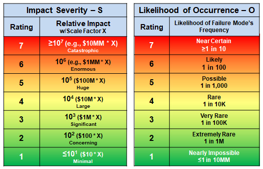
Table 1 – RPN rating tables for impact severity (S) and likelihood of occurrence (O). The severity rating ranges from 1‑minimal to 7‑catastrophic to describe an exponentially increasing magnitude of impact. Likelihood is also rated by an exponential scale of the estimated frequency of the failure mode’s occurrence. While the SME team is free to determine the scales for their analysis, the seven category RPN scales are used in this article to maintain similarity with the following SRS discussion.

In order to prioritize the failure modes, the SME team estimates S and O values for each failure mode and then multiplies them together to calculate the failure mode/effect’s RPN as shown in Table 2.

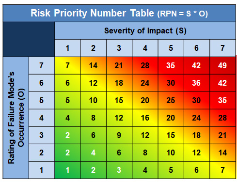
Table 2 – Using the attribute rating scales shown in Table 1, a risk’s S and O attributes are multiplied together to define the effect’s RPN for each failure mode. The above table is frequently called a “heat map” since the higher the RPN, the higher the risk’s priority for remediation.

FMEA’s primary method of controlling risks is to decrease the RPN for an unacceptable risk by either reducing the risk’s severity rating S or decreasing the failure mode’s likelihood of occurrence rating O.

One result of using scalar rating values for S and O is that dissimilar risks can have the same or similar RPN values. For example, a huge (5)/very rare (3) risk with an RPN of 15 is rated similarly to a concerning (2)/near certain (7) risk with an RPN of 14. If risks are prioritized based on RPN, then the two risks might be considered essentially equal, resulting in similar treatment. Close examination of Table 2 shows similar RPN values appearing in many different locations representing potentially dissimilar risks receiving similar scores. Subsequent discussions among the FMEA team members regarding the location of the same or similar RPN values sometimes results in thought‑provoking discussions and disagreements about whether two different risks should receive the same priority or receive the same treatment for possible remediation. Based on the risks being analyzed, it is not unusual for an SME team to significantly alter the specific analysis’ heat maps, like the one shown in Table 2, to satisfy differing opinions on the appropriate priority for specific risks.

With the basic structure of FMEA/RPN defined, we switch to the SRS/ARL approach of understanding and analyzing.

SRS And ARL

While FMEA does not explicitly define a risk, it provides a method of analyzing failure modes of likelihood O that result in an effect of severity S. On the other hand, SRS defines a risk as an input threat (or failure mode) of likelihood L_T entering a system that has a likelihood L_P of not controlling the threat to result in an output risk consequence of severity S_C and a likelihood of L_C. The basic structure of SRSs is shown in Figure 1. The likelihood of the consequence L_C is defined as the mathematical product of L_T and L_P. The likelihood of the threat L_T is estimated by analyzing the previous system that produces the threat. Estimating the likelihood of the threat propagating through the system L_P is accomplished by evaluating the mechanism by which the input threat passes or is propagated through the system to result in the output risk consequence.⁴

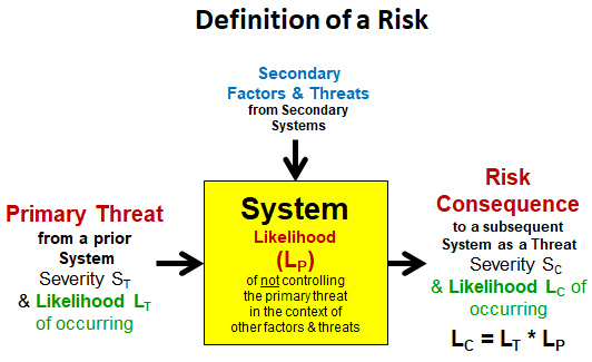
Figure 1 - The basic SRS risk element describes how input threats might propagate or flow through a system to result in output risk consequences. A risk is defined as a possible threat with a likelihood L_T that enters a system that has a likelihood L_P of failing to control the threat to produce a risk consequence of severity S_C and likelihood L_C. As shown, L_C is defined as the mathematical product of L_T and L_P.

The severity of the risk consequence S_C and probability or likelihood of occurrence L_C are described and rated using the tables shown in Table 3.

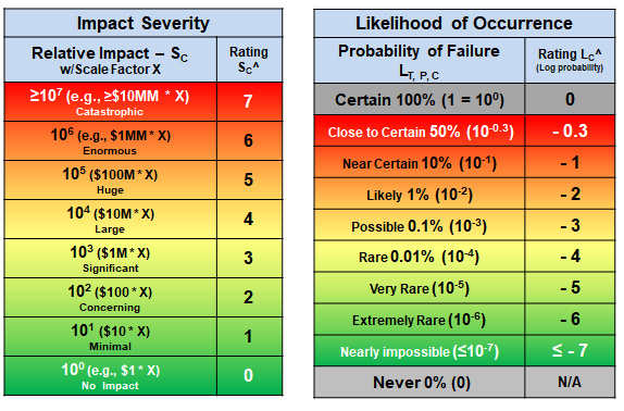
Table 3 – Attribute rating scales for all SRS evaluated risks. The severity table on the left uses a logarithmic scale to provide a seven orders of magnitude range necessary to completely characterize any risk’s impact. The likelihood of occurrence L_C is treated as a probability ranging from certain (100%) to never (0%). The rating for L_C is also a logarithmic scale covering seven orders of magnitude to also cover the complete range for estimating any risk’s probability of occurring.

As shown in Table 3, the severity rating S_C^ is the log of S_C. Similarly, the risk consequence’s likelihood rating L_C^ is the log of L_C. The rating values S_C^ and L_C^ are used in the SRS discussion for convenience as a shorthand for discussing the risk’s attributes. If the ARL is defined as the sum of S_C^ and L_C^ then a single number can be used to quickly characterize a risk. Like the RPN, an ARL table can be constructed as the sum of S_C^ and L_C^ as shown in Table 4.

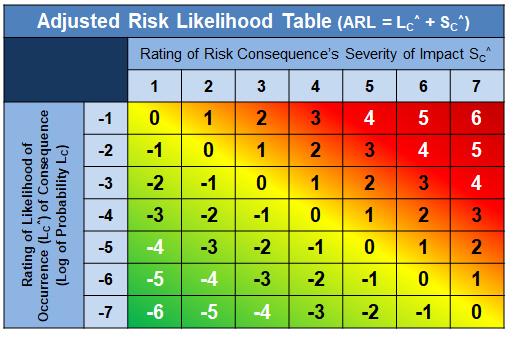
Table 4 – Adjusted risk likelihood (ARL) table created by adding S_C^ and L_C^ together. Because S_C^ and L_C^ are logarithmic representations of S_C and L_C, adding them together is roughly equivalent to the RPN’s approach of multiplying S and O.

Since the heat map shown in Table 4 is balanced around S_C^ = L_C^, the ARL can be effectively described by a simpler representation shown in Figure 2.

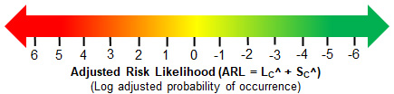
Figure 2 – A simplified representation of SRS’s ARL. While L_C^ and S_C^ should not be combined for analyzing and discussing a risk, the two ratings can be quickly added to gain a concise perspective of the risk’s potential impact.

The ARL provides a convenient method of quickly assessing a risk’s significance. The more positive the ARL value, the more likely the risk will have a significant adverse impact. Conversely, the more negative the ARL, the less likely it will have a significant impact.

Like the RPN, the ARL values can be similar for different risks. However, the ARL values for high impact/low likelihood risks and low impact/high likelihood risks are symmetric. ARL values of zero appear to be a convenient balancing point for many risks. Nevertheless, it can be reasonably argued that a nearly impossible/catastrophic risk is not the same as a nearly certain/minimal‑impact risk even though they both have an ARL value of zero.

The central feature of controlling risks using the SRS method is that risks are mitigated based on their severity S_C^ by reducing either or both L_T and L_P to reduce L_C to an acceptable level. Using the ARL as a guide, the risk consequence’s likelihood L_C should be reduced to a rating value L_C^ that counterbalances the S_C^ rating. In many cases, the ARL value should be near zero or negative.

With the essentials of FMEA and SRS defined, we can compare and contrast the two approaches.

Comparing FMEA/RPN And SRS/ARL

FMEA and SRS have important similarities and differences. The most important similarity is that they both focus on a risk’s cause and effect relationship. FMEA starts with a failure mode having a likelihood of occurrence O described by a scalar integer rating from 1 to N, usually based on a frequency of occurrence as shown in Table 1. Because O is rated as a positive integer, FMEA does not treat the likelihood of occurrence as a probability. Using the lexicon of SRS, FMEA’s failure mode is equivalent to an SRS’s input threat. When using SRS, the O is replaced by the probability L_T as shown in Figure 1.

Both methods use a similar method of rating a risk’s severity. In this article, FMEA rates severity S as shown in Table 1 and SRS’s risk consequence severity rating S_C^ is a scalar integer as shown in Table 3. For FMEA, the severity rating tables range widely based on the judgement and preferences of the SME team. In some cases, the FMEA teams use a linear scale while other teams define a logarithmic scale like the scale shown in Table 1. In the case of SRS, the method defines a single pair of logarithmic scales shown in Table 3 for all risks. The diversity of FMEA rating scales for S and O add considerably to the complexity and difficulty of using and communicating the results of an FMEA, while the uniform, well defined rating scales of L_C and S_C make the SRS approach more universally usable and transferable.

While the SRS approach is designed to start very simply by identifying the threats and risk consequences and then connecting the threats and consequences by systems, the FMEA approach is complicated by a considerable number of specific procedures defined by the team prior to conducting the risk analysis. Well trained and experienced FMEA practitioners can perform effective risk analysis. However, FMEA has proven to be difficult to use for many groups, particularly as a quick method of assessing a specific risk environment. The results of a particular FMEA can also be essentially impossible to communicate to other groups that did not participate in the original risk analysis exercise. These difficulties are well summarized by the following quote from Carlson:⁵

FMEAs, when properly performed on the correct parts with the correct procedure during the correct time frame with the correct team can prevent costly failures before products enter the marketplace. (page 2, italics in the original quote)

In his introduction, Carlson describes the complexity and nonuniversality problems as follows:

FMEA is a broad subject, with a wide variety of standards, procedures, and application. There is no shortage of opinions and ideas from practitioners, both new and experienced. It is impossible to fully satisfy everyone, from every level of experience and every industry and application.⁵ (page xxv, italics added)

FMEA’s complexity is also demonstrated by the FMEA’s risk registers that include numerous columns for S, O, and D rating numbers and category descriptions used by the team to describe and document their consensus for the different risks.⁶

A major difference between FMEA and SRS is their ease and span of application. For example, SRS’s foundational concepts can be used spontaneously to understand safety risks by identifying how threats (hazards) might flow through sequences of systems (risky situations) to result in bad consequences (harm). Driving a car is fundamentally a continuous SRS analysis, with the driver and car identifying threats and using the driver’s skills and the car’s capabilities (the systems) to prevent accidents.⁷ But the same SRS approach described in Figure 1 can be used by a team of experts to understand the input threats that might flow through complex systems to evaluate and, when necessary, manage the likelihood of serious output risk consequences. For example, SRS can easily describe how an individual can use personal protection equipment (PPE) and situational awareness to manage the risk of becoming infected by other people possibly infected with a virus.⁸

The complexity of FMEA frequently results in the method being misapplied or misunderstood. Carlson highlights one of most frequent misapplication of the occurrence rating (O) with the statement:

“Some practitioners attempt to use the occurrence ranking to reflect the likelihood of the effect instead of the likelihood of the cause.”⁵ (page 140, italics in original)

Translating FMEA into SRS terms, the misapplication means that the analysis team is evaluating S_C^ (S) and L_C^ when it should be evaluating S_C^ and L_T^ (O). Carlson’s observation emphasizes that an FMEA is best used as a threat (failure mode) analysis of fragile systems (L_P = 1 or L_P^ = 0; see Table 3). Fragile systems cannot control input threats and thus a realized input failure almost always results in an undesired effect (risk consequence). A television is an example of a fragile system where a single component failure results in a failure of the TV.

Another weakness of FMEA is that it is not structured to handle robust systems. Robust systems have a significant capability of controlling many input threats (L_P^ ≤ -1). An experienced car driver is an excellent example of a robust system.⁷ A risk analysis for a robust system identifies and uses the likelihood of the threat L_T and the likelihood of the system controlling the threat L_P in a straightforward approach to evaluate and manage risks by controlling the likelihood of their occurrence L_C.^7,8

An additional weakness of FMEA is that it is limited to analyzing only one set of risks. FMEA evaluates one layer of input threats (failure modes) to analyze one layer of risk consequences (effects). Because FMEA does not treat likelihood of occurrence as a probability, it is unable to transparently deal with the interactive nature of multiple sequential systems. SRS, however, is designed to couple the risk elements shown in Figure 1 into sequences of systems to describe how threats flow through and can be controlled by multiple systems. This capability also facilitates dividing complex systems into subsystems. For a complex risk analysis, the SRS risk element shown in Figure 1 can also be used to form networks to describe and understand how multiple input threats might impact the likelihood of a risk consequence.

Perhaps SRS’s greatest long-term advantage over FMEA is the ability to manage both risks and benefits.⁹ Since a broader definition of a risk, such as the definition in ISO 31000 – “the effect of uncertainty on objectives”¹⁰ merges risks and benefits, a complete risk analysis method should be able to simultaneously manage both risks and benefits. Benefits, like risks, can be described by a fairly straightforward cause and effect relationship requiring both the likelihood of occurrence and level of impact to be identified and described as shown in Figure 1. If the benefit is described as the combination of a benefit severity rating S_B^ and likelihood rating of L_B^, then a broader characterization of a risk might be the risk benefit score (RBS), calculated as (S_B^ - S_C^) + (L_B^ - L_C^).⁹ A complete method for using SRS to simultaneously understand and manage risks and benefits remains, at this point in time, for the future.

Conclusion

While FMEA can be a useful risk analysis method, SRS is more useful because it better describes both a specific risk element and how sequences and networks of risk elements can be combined to describe and understand more complex risk situations. SRS also treats likelihoods as probabilities instead of subsuming likelihoods as a weighting factor to the risk’s severity rating. Using the complete SRS risk definition, FMEA can be shown to be a limited subset of the SRS approach. FMEA contains imbedded assumptions about the systems it analyzes that limit its ability to completely describe many risk situations. While FMEA has been historically difficult to use, the SRS approach’s simple terminology and universal attribute scales provide a straightforward paradigm for executing and documenting risk analysis and management exercises.

References

1. FDA (CDER/CBER) – Guidance for industry: Q9 quality risk management, June 2006. ICH.
2. Box G. & Draper N., Empirical Model Building and Response Surface, Wiley, 1987.
3. Witcher, M.F., Rating Risk Events: Why Adjusted Risk Likelihood (ARL) Should Replace Risk Priority Number (RPN), BioProcess Online, April 7, 2021. https://www.bioprocessonline.com/doc/rating-risk-events-why-we-should-replace-the-risk-priority-number-rpn-with-the-adjusted-risk-likelihood-arl-0001
4. Witcher, M.F. – Estimating the uncertainty of structured pharmaceutical development and manufacturing process execution risks using a prospective causal risk model (PCRM). BioProcess J. 2019; 18. https://doi.org/10.12665/J18OA.Witcher
5. Carlson, C., Effective FMEAs – Achieving Safe, Reliable, and Economical Products and Processes Using Failure Mode and Effects Analysis, Wiley, 2012.
6. McDermott R., et.al., The Basics of FMEA, Productivity Press, 1996.
7. Witcher, M.F., System Risk Structures: A New Framework for Avoiding Disaster, BioProcess Online, July 13, 2020. https://www.bioprocessonline.com/doc/system-risk-structures-a-new-framework-for-avoiding-disaster-by-managing-risks-0001
8. Witcher, M.F., What Managing Personal SARS-CoV-2 Risks Can Teach Us About Managing Pharma Risks, BioProcess Online, June 12, 2020. https://www.bioprocessonline.com/doc/what-managing-personal-sars-cov-risks-can-teach-us-about-managing-pharma-risks-0001
9. Witcher, M.F., Using System Risk Structures to Understand and Balance Risk/Benefit Trade-off, BioProcess Online, April 23, 2021. https://www.bioprocessonline.com/doc/using-system-risk-structures-to-understand-and-balance-risk-benefit-trade-offs-0001
10. ISO 31000:2018 – Risk Management – International Organization for Standardization.

About The Author:

Mark F. Witcher, Ph.D., is a bioprocess operations expert with 35 years of experience in the biopharmaceutical industry in a wide variety of executive, consulting, and engineering roles. Previously, Mark was a member of NNE’s Strategic Manufacturing Concept Group after working at IPS on feasibility and conceptual design studies for advanced biopharmaceutical manufacturing facilities. He has more than 25 years of experience as a consultant in the biopharmaceutical industry on operational issues related to product development, process validation, strategic business development, clinical and commercial manufacturing planning, tech transfer, and facility design. He was previously senior vice president of operations at Covance Biotechnology Services and vice president of manufacturing at Amgen, Inc.